Ptolemaics meetings 4 & 5 & 6 ; pt I

These last ones have been quite interesting meetings, I’m happy about how the whole thing is turning out. Sadly I’m very slow at typing and working out the ideas, so I have to include three different meetings in one. Since the notes are getting incredibly long, I’ll have to split it in at least two parts.I include the pdf version of it, in case it makes it any easier to read.

ptolemaics meeting 4 & 5 & 6 pt I

Let me get finally into the time frequency of the Walsh phase plane. I won’t include many proofs as they are already well written in Hytönen’s notes (see previous post). My main interest here is the heuristic interpretation of them (disclaimer: you might think I’m bullshitting you at a certain point, but I’m probably not). Ideally, it would be very good to be able to track back the train of thoughts that went in Fefferman’s and Thiele-Lacey’s proofs.

Sorry if the pictures are shit, I haven’t learned how to draw them properly using latex yet.

1. Brush up

Recall we have Walsh series for functions ${f \in L^2(0,1)}$ defined by

$\displaystyle W_N f(x) = \sum_{n=0}^{N}{\left\langle f,w_n\right\rangle w_n(x)},$

the (Walsh-)Carleson operator here is thus

$\displaystyle \mathcal{C}f(x) = \sup_{N\in \mathbb{N}}{|W_N f(x)|},$

and in order to prove ${W_N f(x) \rightarrow f(x)}$ a.e. for ${N\rightarrow +\infty}$ one can prove that

$\displaystyle \|\mathcal{C}f\|_{L^{2,\infty}(0,1)} \lesssim \|f\|_{L^2(0,1)}.$

There’s a general remark that should be done at this point: the last inequality is equivalent to

$\displaystyle \left|\left\langle\mathcal{C}f, \chi_E\right\rangle\right| = \left|\int_{E}{\mathcal{C}f}\,dx\right| \lesssim |E|^{1/2}\|f\|_{L^2(0,1)}$

to hold on every measurable ${E}$ (of finite measure).
This is because in general an estimate of the kind

$\displaystyle \left|\{x\,:\, |Tf|>\lambda\}\right|\lesssim \frac{\|f\|_{L^p}^q}{\lambda^q}$

is equivalent to

$\displaystyle \left|\int_{E}{Tf}\right|\lesssim \|f\|_{L^p}|E|^{1/q^\prime} \quad\quad\quad \forall \text{ measurable } E.$

To see why, suppose the first is true and take ${E}$ arbitrary: then by triangular inequality for the integral it is equivalent to estimate

$\displaystyle \sum_{k}{2^k \left|\{x\in E\,:\, |Tf|\sim 2^k\}\right|} =: \sum_{k}{2^k \left|E_k\right|},$

and we easily have ${|E_k|\leq \min\{|E|, 2^{-qk}\|f\|_{L^p}^q\};}$ the second then follows by summing (optimize according to this last inequality). Now if you suppose the second one is true instead, and consider positive/negative parts of real/imaginary parts of ${Tf}$ , you just have to take ${E \subset \{x\,:\, |Tf|>\lambda\}}$ of finite measure, and let it approach the whole set. It follows immediately that the first one holds.

So, we can content ourselves with proving

$\displaystyle \left|\int_{E}{\mathcal{C}f}\,dx\right| \lesssim |E|^{1/2}\|f\|_{L^2(0,1)}.$

2. Walsh wave packets

In the previous post I’ve stated some properties of the Walsh functions, one of which was that if ${m \oplus n = m + n }$ (i.e. their binary digits are complementary when overlapping) then

$\displaystyle w_{m+n} = w_m \cdot w_n.$

It’s actually true in general, by what seen in previous post, that

$\displaystyle w_{m\oplus n} = w_m \cdot w_n.$

Now, the Walsh functions are an orthonormal basis for ${L^2(0,1)}$ , thus if you consider functions as linear combinations of Walsh functions, multiplying by ${w_m}$ is equivalent to “shifting” by ${\oplus m}$ the indices of the Walsh functions that compose ${f}$ – or equivalently to shift the Walsh transform ${Wf}$ by ${\oplus m}$ . Bear in mind the field ${\mathbb{Z}_2 [[X]]}$ has order two, so shifting in this setting doesn’t necessarily resemble shifting in ${\mathbb{R}}$ . Anyhow, from the group point of view, this is analogous to what happens when you modulate an ${L^2(\mathbb{R})}$ function by ${e^{2\pi i x \eta}}$ : you’re shifting its Fourier transform by ${\eta}$ . Modulation in time equals translation in frequency and viceversa. Hence we can follow the analogy and consider the phase-plane point of view on the Walsh transform. This is just ${\mathbb{Z}_2 [[X]] \times \mathbb{Z}_2 [[X]]}$ .

We need to introduce wave packets associated to rectangles ${I \times \omega}$ according to the principle that the time interval ${I}$ contains information about the time localization, and ${\omega}$ about the frequency. Define thus the packets as

$\displaystyle w_{I\times \omega} (x) = \underbrace{\frac{1}{|I|^{1/2}}}_{L^2\text{ norm. factor}} \cdot \underbrace{\chi_{I}(x)}_{\text{time localization}} \cdot \underbrace{e\left(\frac{x \otimes (|I|\xi_\omega)}{|I|}\right),}_{\text{freq. modulation}}$

where ${\xi_\omega}$ is the left endpoint of ${\omega}$ .

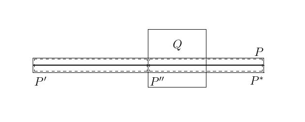
We look a bit more in detail into the localization properties of such wavepackets. Notice that if ${\xi_\omega=0}$ then it is just ${|I|^{-1/2}\chi_I}$ . Its Walsh-Fourier transform is

$\displaystyle |I|^{-1/2}\widehat{\chi_I}(\xi) = |I|^{-1/2}\int_{I}{e(x\otimes \xi)}\,dx =|I|^{-1/2}e(x_I \otimes \xi) \int_{0}^{|I|}{e(x\otimes \xi)}\,dx,$

and the value of the integral is calculated as follows: it is

$\displaystyle a_{-1}(x\otimes \xi) = \sum_{m+n=-1}{x_m \xi_n} \mod \mathbb{Z}_2,$

where on the integration interval ${x_m \equiv 0}$ for ${m\geq \log_2 |I|}$ ; it follows that the integral factor is constant in ${\xi}$ on intervals of size ${2^{-\log_2 |I|} = |I|^{-1}}$ . If ${\xi}$ is ${\neq 0}$ then ${e(x\otimes \xi)}$ will be ${+1}$ half of the times on ${[0,|I|]}$ , and ${-1}$ the rest of the times, so that the interval is zero. On the contrary, if ${\xi = 0}$ then the integral is ${|I|}$ . Summarizing

$\displaystyle |I|^{-1/2}\widehat{\chi_I}(\xi) = |I|^{1/2} \chi_{[0,|I|^{-1}]}(\xi) e(x_I \otimes \xi).$

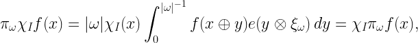
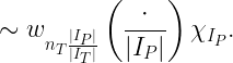
This is remarkable: the Walsh-Fourier transform is still localized! This means that the frequency projection multiplier

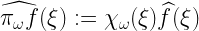
$\displaystyle \widehat{\pi_\omega f}(\xi) := \chi_\omega(\xi) \widehat{f}(\xi)$

is convolution with

$\displaystyle |\omega|\, \chi_{[0,|\omega|^{-1}]}(x)\, e(x \otimes \xi_\omega).$

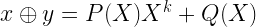
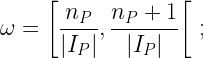
Remark 1 Let’s make clear what a dyadic interval is, given the mapping between reals and Laurent series. Given a dyadic interval ${[j 2^k, (j+1) 2^k[}$ , let ${P(X)}$ be the polynomial representation of ${j}$ ; then the interval on ${\mathbb{Z}_2 [[X]]}$ contains all the polynomials of the form ${P(X)X^k + Q(X)}$ , where ${Q(X)}$ is any Laurent series with ${\deg (Q) < k}$ .

2.1. Uncertainty Principle in the Walsh phase-plane

We are tempted to localize both in time and frequency in the Walsh plane. If we do so, we obtain

$\displaystyle \pi_\omega \chi_I f (x) = |\omega| \int_{0}^{|\omega|^{-1}}{\chi_I(x\oplus y) f(x \oplus y) e(y\otimes \xi_\omega)}\,dy.$

Look at the characteristic function inside the integral. For that to be ${=1}$ , it must be ${x\oplus y = P(X)X^k + Q(X)}$ , where ${|I|=2^k}$ , and ${\deg (Q) < k}$ . On the other hand ${y}$ is of the form ${Q(X)}$ with ${\deg Q < -l}$ , where ${|\omega|=2^\ell}$ . If we assume ${-\ell \leq k}$ something magic happens:

$\displaystyle x\oplus y \in I \Leftrightarrow x \in I \quad !$

This is because the degree of ${y}$ is too small to affect the sum ${x \oplus y}$ , relatively to ${I}$ . This means that if ${|I| |\omega|\geq 1}$ then ${\chi_I}$ factors out of the integral, and the expression becomes

$\displaystyle \pi_\omega \chi_I f (x) = |\omega| \chi_I (x) \int_{0}^{|\omega|^{-1}}{f(x\oplus y) e(y\otimes \xi_\omega)}\,dy = \chi_I \pi_\omega f (x),$

i.e. if the tile ${I\times \omega}$ has area 1, then the associated time and frequency localizations commute with each other! Let me state that once again:

$\displaystyle |I||\omega| \geq 1 \quad \quad \Rightarrow \quad \quad \pi_\omega \chi_I = \chi_I \pi_\omega.$

Remark 2 This NEVER EVER happens in the real case, as ${\chi_I\pi_\omega f}$ has bounded support, while ${\pi_\omega \chi_I f}$ has unbounded support (because its Fourier transform has bounded support).

Why is this relevant to us though? well, ${\chi_I}$ and ${\pi_\omega}$ are projections and in particular they are self-adjoint; commutativity ensures both that the operator ${\pi_\omega \chi_I}$ is self-adjoint, and that it is idempotent. Therefore ${\pi_\omega \chi_I}$ is a projection operator. See below for how is this related to the wavepackets.

Anyway, what happened there? That’s the Uncertainty Principle at work. It’s lurking behind the tiles, and it suggests us to restrict our attention to tiles ${P}$ of area ${\geq 1}$ . Actually it’s best to restrict ourselves to only consider tiles of area exactly ${1}$ (so that they are “critical”). The reason for that is that if we assume area ${1}$ (or constant, in general) then there is a 1-to-1 correspondence between areas of the phase-plane (made of tiles) and the linear spans of the wavepackets associated to those tiles. This might sound confusing, so I will restate it properly in a moment; I need to fix some definitions first.

DISCLAIMER: from now on, by tile I mean a dyadic rectangle with area 1. Since it will be useful, I will also introduce bi-tiles, which are dyadic rectangles of area 2. In particular, if you split a bi-tile ${P}$ in two halves horizontally, then you get two tiles, the lower half being denoted ${P_d}$ and the upper half ${P_u}$ .

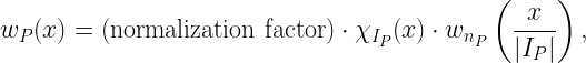
Let’s rewrite the expression for the wavepackets: since ${|I_P||\omega_P| =1}$ , there’s an integer ${n_P}$ such that we can write

$\displaystyle \omega = \left[\frac{n_P}{|I_P|}, \frac{n_P + 1}{|I_P|}\right[\,;$

then the wavepacket associated to ${P}$ is

$\displaystyle w_P (x) := \frac{1}{|I_P|^{1/2}}\; \chi_I (x) \; w_{n_P}\left(\frac{x}{|I_P|}\right).$

For example,

$\displaystyle w_{[0,1]\times [n,n+1[}(x) = w_n (x).$

It’s also easy to see that if $P$ , $Q$ are disjoint tiles, then

$\displaystyle \left\langle w_P, w_Q\right\rangle = 0.$

The operators ${\pi_\omega \chi_I}$ deserve their definition as well, and we write

$\displaystyle \Pi_P := \pi_{\omega_P} \chi_{I_P}$

for the phase projection.

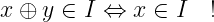
The property we just mentioned above is the fact that given two collections of tiles ${\mathbb{P}}$ and ${\mathbb{Q}}$ , the spans of the ${w_P}$ ‘s and ${w_Q}$ ‘s will coincide. In detail, the following holds:

Proposition 1 If ${\mathbb{P}}$ is a collection of tiles and ${Q}$ is a tile such that

$\displaystyle Q \subset \bigcup_{P\in\mathbb{P}}{P},$

then

$\displaystyle w_Q \in \mathrm{Span}\{w_P\,:\, P\in\mathbb{P}\}.$

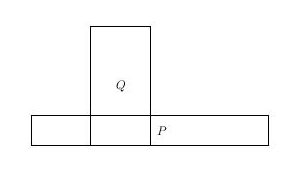
The proof is easy and works out thanks to the combinatorics of the dyadic intervals, and the following elementary fact: the tiles in this picturehave the same span as the tiles in this picture provided they cover the same portion of the phase-plane.

Proof: Suppose ${Q}$ is not contained in ${\mathbb{P}}$ otherwise it’s all trivial. First of all discard all the unnecessary tiles in the collection. We know that wavepackets with disjoint tiles are orthogonal to each other, so that we can forget about the tiles in ${\mathbb{P}}$ that don’t intersect ${Q}$ – i.e. assume all of them do intersect ${Q}$ . We can then discard some more tiles actually, and be left with a minimal collection ${\mathbb{P}}$ that covers ${Q}$ but is made only of vertical tiles (i.e. with ${I_P \subset I_Q}$ and then ${\omega_P \supset \omega_Q}$ because the area is constant) or horizontal ones (the opposite of vertical). This is because a vertical tile necessarily covers an entire strip (here we’re using the constant area hypothesis!), since ${\omega \supset \omega_Q}$ : then if a point ${(x,y)\in Q}$ is not covered by vertical tiles, all of ${\{x\}\times \omega_Q}$ is not covered. Thus the strip must be covered by horizontal ones, and those have a time interval larger than ${I_Q}$ ! therefore they cover all of ${Q}$ and you can forget about the vertical ones (same thing works in the other way).

At this point, assuming only a minimal cover of horizontal tiles, we’re halfway done: call ${P}$ the widest one and ${P^\ast := I_P \times \omega_P^\ast}$ , where ${\omega_P^\ast}$ is the sibling of ${\omega_P}$ ; then ${P^\ast \cap Q \neq \emptyset}$ as well (by nestedness of the dyadic intervals), and ${P^\ast}$ must belong to the collection too, since if the area ${I\times \omega_P^\ast}$ were covered by a tile shorter than ${P}$ , this tile would cover ${P\cap Q}$ as well, which contradicts minimality. Thus we have a couple of congruent tiles ${P,P^\ast}$ , both contained in the collection. By the remark stated before this proof, we can substitute ${P,P^\ast}$ with the tiles ${P', P''}$ as in figure, without altering the span; but if ${P}$ is wider than ${Q}$ then only one of these tiles will intersect ${Q}$ (tile ${P''}$ in the figure), so we can discard the other one.

Now one applies this step inductively and gets an algorithm that stops once it gets to the full tile ${Q}$ , which then belongs to the span of ${\mathbb{P}}$ . $\Box$

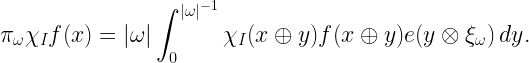
I think the above arguments should provide sufficient motivation for the choice of wavepackets associated to tiles of area 1. As a further remark, I would like to point out that the choice of the particular expression for the wavepackets is absolutely natural once the above phase projections have been taken into consideration. As a matter of fact, as one can imagine, all the projections ${\Pi_P}$ can be obtained one from the other by translations, modulations and scaling. In particular one can concentrate on the simplest one, namely for ${P_0 = [0,1]\times [0,1]}$ , and see that

$\displaystyle \Pi_{P_0}f = \chi_{[0,1]} (x) \int_{0}^{1}{f(x\oplus y)}\,dy,$

and given the first factor in the RHS we see that this is equal to

$\displaystyle \Pi_{P_0}f = \chi_{[0,1]} (x) \left(\int_{0}^{1}{f}\right),$

i.e. the ${\Pi_P}$ ‘s have all rank 1. This is remarkable, because it tells us there’s a function ${\phi_P}$ such that for ${f\in L^2}$

$\displaystyle \Pi_P f = \left\langle \phi_P, f \right\rangle \phi_P;$

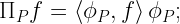
in the above case it is

$\displaystyle \phi_{[0,1]\times [0,1]} = \chi_{[0,1]}.$

What is ${\phi_P}$ ? well, we can obtain it by translation modulation and scaling of the above ${\phi_{[0,1]\times [0,1]}}$ , and what we get is

$\displaystyle \phi_P (x)= \frac{1}{|I_P|} \chi_{I_P}(x) e(|I_P|^{-1} x \otimes \xi_{\omega_P}),$

which is exactly the wavepacket ${w_P}$ !

3. Rewriting ${W_N}$ in a useful form

How do we exploit the phase-plane structure efficiently? well, first of all we need to write ${W_N f(x)}$ in terms of wavepackets. By definition the Walsh function of index ${n}$ restricted to the interval ${[0,1]}$ is the wavepacket of tile

$\displaystyle [0,1] \times [n,n+1[,$

and therefore

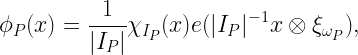
$\displaystyle W_N f(x) = \sum_{P\,:\,I_P=[0,1], \omega_P \subset [0,N]}{\left\langle f, w_P\right\rangle w_P(x)}.$

Thus it is a projection onto a subspace of wavepackets. This collection of tiles is a very lame and uninteresting one though – just some squares stacked on top of each other. What will happen if we change the set of tiles? well, as the proposition above tells us, as long as the tiles cover the same area in the phase-plane, the linear spans of the associated wavepackets are exactly the same. And since the operator is a projection and the wavepackets are orthogonal (if the corresponding tiles are disjoint), it follows that the operator will stay the same if the tilings are collections of disjoint tiles!

Therefore, we look for another cover of the rectangle ${[0,1]\times [0,N]}$ . To find one, we use an idea that already appeared in the first post of this series. Let me recall it briefly: we had an integral on an interval ${]-\infty, \alpha]}$ and a dyadic system on ${\mathbb{R}}$ (doesn’t matter which particular one); we wanted to decompose it into a sum of integrals ${\int_\omega}$ where ${\omega}$ was a generic dyadic interval in the system. What we did was to write

$\displaystyle \int_{]-\infty, \alpha]}{f} = \sum_{\omega_\ell \text{ s.t. } \omega_r \ni \alpha}{\int_{\omega_\ell}{f}},$

i.e. we sum on all left halves of dyadic intervals such that the right half contains ${\alpha}$ .

We now do the analogue in this case: we are interested in bitiles ${P}$ (which correspond to the ${\omega}$ ‘s) such that the upper half ${P_u}$ contains the frequency ${N}$ – or, to be precise, ${N\in \omega_{P_u}}$ . The further condition is that the tiles have time support in ${[0,1]}$ obviously. And then we sum in the lower tiles ${P_d}$ . In formulas

$\displaystyle \sum_{Q\text{ s.t. } I_Q=[0,1], \omega_Q \subset [0,N]} = \sum_{P_d \text{ s.t. } I_P \subseteq [0,1],\, \omega_{P_u} \ni N}$

(notice on the left ${Q}$ is a tile, while ${P}$ on the right is a bitile). The partial Walsh-series is now

$\displaystyle W_N f (x) = \sum_{P_d \text{ s.t. } I_P \subseteq [0,1],\, \omega_{P_u} \ni N}{\left\langle f, w_{P_d}\right\rangle w_{P_d}}.$

Pretty neat! Now the time support of the tiles is allowed to be smaller than ${[0,1]}$ , there’s more freedom to generalize. It takes a little to realize what kind of partition we get, so here’s a picture to help your intuition:

On the left the original tiling for N=7. On the right, the new tiling.

We are ultimately interested in estimating the size of ${\left\langle \mathcal{C}f, \chi_E\right\rangle}$ ; recall the other important idea introduced in the first post of this series: linearization of the supremum! It means we rather want to prove an estimate

$\displaystyle \left|\left\langle W_{N(\cdot)}f, \chi_E\right\rangle\right|\lesssim \|f\|_{L^2} |E|^{1/2}$

uniformly in the measurable function ${N(x)}$ . That means we want to estimate

$\displaystyle \int_{E}{W_{N(x)} f (x)}\,dx = \int_{E}{\sum_{P_d \text{ s.t. } I_P \subseteq [0,1],\, \omega_{P_u} \ni N(x)}{\left\langle f, w_{P_d}\right\rangle w_{P_d}(x)}}\,dx;$

$\displaystyle = \int_{E}{\sum_{P_d \text{ s.t. } I_P \subseteq [0,1]}{\left\langle f, w_{P_d}\right\rangle w_{P_d}(x) \chi_{\omega_{P_u}}(N(x))}}\,dx$

we introduce sets

$\displaystyle E_P = E \cap N^{-1}(\omega_{P_u})$

so that we can write the last integral as

$\displaystyle \sum_{P_d \text{ s.t. } I_P \subseteq [0,1]}{\left\langle f, w_{P_d}\right\rangle \left\langle w_{P_d}, \chi_{E_P}\right\rangle}.$

The sets ${E_P}$ contain exactly those points in ${E}$ such that ${N(x) \in \omega_{P_u}}$ as required. Now, the collection of bitiles ${P}$ with time support ${\subset [0,1]}$ have nothing special; therefore we will work in general with the sums

$\displaystyle \sum_{P \in \mathbb{P}}{\left\langle f, w_{P_d}\right\rangle \left\langle w_{P_d}, \chi_{E_P}\right\rangle}, \quad \quad \quad \quad \quad (\clubsuit)$

where ${\mathbb{P}}$ is any collection of bitiles in the Walsh phase-plane. Our estimates will need to be uniform in ${\mathbb{P}}$ of course, but the freedom this gives is worth the trouble.

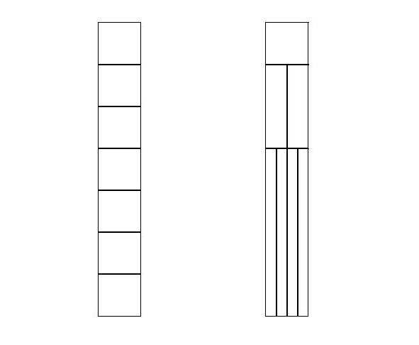
4. Trees of tiles

In his seminal proof, Fefferman introduced a particular structure on tiles: the Tree. The definition requires a partial ordering on the bi-tiles (or tiles), which is as follows: given tiles ${P, Q}$ , it is

$\displaystyle P \succeq Q$

if and only if

$\displaystyle I_P \supset I_Q \mbox{ and }\omega_P \subset \omega_Q$

(thus they intersect, and the one with smaller time support is the “smaller” one).

Here P>Q

Then we say that a finite collection of bi-tiles ${\mathbb{T}}$ is a tree with top bi-tile ${T \in \mathbb{T}}$ if and only if

$\displaystyle P \preceq T \quad \quad \quad \forall P \in \mathbb{T}.$

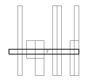
This is a tree with top bi-tile T (the thickened one).}

One has the notions of up-tree and down-tree requiring respectively that ${P_u \preceq T_u}$ and ${P_d \preceq T_d}$ (so, the upper half of the collection is a tree, or the lower half). It is possible to decompose every tree in its up-tree and down-tree part (the share the top tile, but only that); for example, for the tree in figure one has the following decomposition:

This is the up-tree part of T

This is the down-tree part of T.

I think of trees as clumps of narrow elongated tiles that intersect a single larger tile – the top tile, or root. Notice an up-tree is a more concentrated clump, as the upper half of any tile in the tree still has to intersect (the upper half of) the top tile, so that the center of the frequency support of any tile in the tree cannot be too far from that of the top tile ${T}$ . This is not necessarily true of a down-tree, as it can contain very narrow and tall tiles, with the frequency support potentially unbounded. The figure I’ve included should make it clearer.

On the left, a typical down-tree. On the right, a typical up-tree.

The useful lemma that follows highlights the pros of the up-tree structure and takes to a conclusion the idea I’ve just sketched:

Lemma 2 Let ${\mathbb{T}}$ be an up-tree with top tile ${T}$ . Then for every (up-)leaf ${P \in \mathbb{T}}$ we can write ${w_P}$ in terms of ${w_T}$ as follows:

$\displaystyle w_{P_d} (x) = \epsilon_{P,T} \frac{1}{|I_T|^{1/2}}\;w_{T_u} (x)\; h_{I_P}(x),$

with ${\epsilon}$ ‘s some signs ${\pm}$ that depend on the tiles and ${h_{I_P}}$ the Haar function supported on the interval ${I_P}$ ( ${L^2}$ normalized as it’s customary).

The proof can be obtained just by unwinding the definitions, but that doesn’t say much about it. Here’s why we should expect something like the above to hold. ${P}$ being a leaf means just that ${P_u \leq T_u}$ , and in particular that they intersect (and ${P}$ is taller than ${T}$ , and away from the zero frequency as well – this is important) both in time and frequency. Thus it should be

$\displaystyle c(\omega_P) \sim c(\omega_T)$

(notation: ${c(I)}$ is the center of the interval ${I}$ ; we also ignore the pedices to ease reading), which means that the ratios ${\text{frequency}/\text{support size}}$ should be comparable, namely

$\displaystyle \frac{n_T}{|I_T|}\sim\frac{n_P}{|I_P|}.$

(for a down-tree you could only say ${c(\omega_P) \gtrsim c(\omega_T)}$ .)

You can think of ${n_P}$ as the “number of times ${w_P}$ oscillates” (a frequency indeed). By the above we expect ${w_P}$ to oscillate about ${\frac{|I_P|}{|I_T|}n_T}$ times. We also know it is supported in ${I_P}$ . Think of it in a purely probabilistic perspective: ${w_T}$ oscillates about ${n_T}$ times within an interval of length ${|I_T|}$ , ${P}$ is a tile roughly in the same location on the phase plane but with smaller support, of size ${|I_P|}$ . We can naively expect ${w_P}$ is almost a restriction of ${w_T}$ on support ${I_P}$ , so that it will capture only a fraction of about ${\frac{|I_P|}{|I_T|}}$ of the oscillations of ${w_T}$ . The lemma is saying that this perspective is not completely wrong indeed.

By definition of wave packet it is

$\displaystyle w_P (x) = (\text{normalization factor})\cdot \chi_{I_P}(x) \cdot w_{n_P}\left(\frac{x}{|I_P|}\right),$

so we expect ${w_P}$ could be expressed by (ignoring normalization factors)

$\displaystyle \sim w_{n_T \frac{|I_P|}{|I_T|}}\left(\frac{\cdot}{|I_P|}\right) \chi_{I_P}.$

In general it is 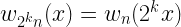${w_{2^k n}(x) = w_{n}(2^k x)}$ , and we can pretend that “morally” this holds for negative ${k}$ as well (it does if the resulting index is integer), so that since the lenghts are powers of 2

$\displaystyle w_{n_T \frac{|I_P|}{|I_T|}}\left(\frac{\cdot}{|I_P|}\right) \chi_{I_P} \sim w_{n_T}\left( \frac{|I_P|}{|I_T|}\frac{\cdot}{|I_P|}\right) \chi_{I_P} \sim w_T(\cdot) \chi_{I_P}.$

This is exactly what I said above: naively one expects ${w_P}$ to be just ${w_T\cdot \chi_{I_P}}$ ! By the above lemma it is almost so, the main difference being that we have ${h_{I_P}}$ instead of ${\chi_{I_P}}$ , which has the effect of changing the sign on the right half of the support, and ${T_u}$ in place of ${T}$ . As a last remark on the above equality, the lemma says that the factor ${w_{T_u}}$ accounts for all oscillation in an up-tree.

So, the notion of tree has some advantages, namely that the wave packets are all essentially restrictions of the top tile’s one, and calculations seem to be more easily carried over on trees (judging by the notes). But I don’t find this answer satisfactory enough: why should we care for trees in the first place?

A better answer is that trees are associated to operators that are Calder\'{o}n-Zygmund like. We’ve considered orthogonal projections of the form

$\displaystyle \sum_{P\in\mathbb{P}}{\left\langle f, w_{P_d}\right\rangle w_{P_d}},$

and it is therefore natural to consider weighted projections of the form

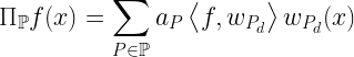
$\displaystyle \Pi_{\mathbb{P}}f(x) = \sum_{P\in\mathbb{P}}{a_P \left\langle f, w_{P_d}\right\rangle w_{P_d} (x)}$

for some weights ${a_P}$ . These operators are bounded on ${L^2}$ for ${\ell^2}$ weights, as it can be easily verified that

$\displaystyle \|\Pi_{\mathbb{P}}\|_{L^2\rightarrow L^2} \lesssim \left(\sum_{P\in\mathbb{P}}{|a_P|^2}\right)^{1/2}.$

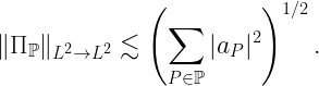
Now, as we did for the euclidean Fourier transform, this can be rewritten as

$\displaystyle \Pi_{\mathbb{P}}f (x) = f \underline{\ast} \left(\sum_{P\in \mathbb{P}}{a_P w_{P_d}}\right)(x),$

where ${\underline{\ast}}$ is the convolution w.r.t. to ${\oplus}$ . Now, suppose ${\mathbb{P}}$ is an up-tree, so that the above lemma applies, and all the wave packets simplify to

$\displaystyle \Pi_{\mathbb{P}}f = f \underline{\ast} \left(\frac{w_{T_u}}{|I_T|^{1/2}}\sum_{P\in\mathbb{P}}{\epsilon_{P,T} a_P h_{I_P}}\right).$

Forget about the signs ${\epsilon}$ ‘s since we can incorporate them into the weights; we now have as a kernel of ${\Pi_{\mathbb{P}}}$ the product

$\displaystyle \frac{w_{T_u}}{|I_T|^{1/2}}\sum_{P\in\mathbb{P}}{a_P h_{I_P}},$

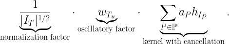
where the only phase factor is ${w_{T_u}}$ and the terms in the sum show very little oscillation: it is just a linear combination of Haar functions with support contained in ${I_T}$ . They correspond to the tiles of the form ${I \times \left[|I|^{-1}, 2|I|^{-1}\right[}$ , which are sometimes called lacunary tiles. Moreover, the function ${\sum_{P\in\mathbb{P}}{a_P h_{I_P}}}$ has zero mean on ${I_T}$ and all the terms are supported in ${I_T}$ by definition of up-tree. So, the kernel is

$\displaystyle \underbrace{\frac{1}{|I_T|^{1/2}}}_{\text{normalization factor}} \cdot \underbrace{w_{T_u}}_{\text{oscillatory factor}}\cdot \underbrace{\sum_{P\in\mathbb{P}}{a_P h_{I_P}}}_{\text{kernel with cancellation}}.$

This operator is thus the analogue in the Walsh setting of something like

$\displaystyle \underbrace{e^{-2\pi i C x}}_{\text{oscillatory factor}}\cdot \underbrace{Q(x)}_{\text{kernel with cancellation}},$

which falls under the scope of Calderón-Zygmund theory. It is a particular case of the case treated in

Ricci, Stein, “Harmonic analysis on nilpotent groups and singular integrals I: oscillatory integrals”, Jour. of Func. Analysis, 73, pg 179-194 (1987)

which is, kernels of the kind

$\displaystyle e^{-2\pi i P(x,y)} K(x-y)$

with ${P}$ a polynomial and ${K}$ a homogeneous kernel of critical degree ${-n}$ (the dimension) and zero average on the sphere. I was planning to write about that paper anyway (half of the blog entry is already there), so stay tuned if you are interested.

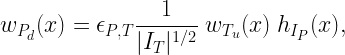
Resuming, the operator of weighted projection associated to an up-tree is a Calder\'{o}n-Zygmund object, and as such we expect that standard techniques will apply to bound it properly (it is indeed so). For a down-tree we don’t have such a nice formula as for the up case, and indeed one can figure out that once the tiles in the down-tree get very narrow, their frequency must be ${0}$ ; we correspondingly expect that there’s no cancellation to exploit in these operators, and as a matter of fact this is indeed the case, as we will see in the following part of these notes.

Enough for today.

Almost Originality

a mathematical journal

Ptolemaics meetings 4 & 5 & 6 ; pt I

Leave a comment Cancel reply

Share this:

Related

Leave a comment Cancel reply