Representing points in a set in positional-notation fashion (a trick by Bourgain): part I

If you are reading this blog, you have probably heard that Jean Bourgain – one of the greatest analysts of the last century – has unfortunately passed away last December. It is fair to say that the progress of analysis will slow down significantly without him. I am not in any position to give a eulogy to this giant, but I thought it would be nice to commemorate him by talking occasionally on this blog about some of his many profound papers and his crazily inventive tricks. That’s something everybody agrees on: Bourgain was able to come up with a variety of insane tricks in a way that no one else is. The man was a problem solver and an overall magician: the first time you see one of his tricks, you don’t believe what’s happening in front of you. And that’s just the tricks part!

In this two-parts post I am going to talk about a certain trick that loosely speaking, involves representing points on an arbitrary set in a fashion similar to how integers are represented, say, in binary basis. I don’t know if this trick came straight out of Bourgain’s magical top hat or if he learned it from somewhere else; I haven’t seen it used elsewhere except for papers that cite Bourgain himself, so I’m inclined to attribute it to him – but please, correct me if I’m wrong.
Today we introduce the context for the trick (a famous lemma by Bourgain for maximal frequency projections on the real line) and present a toy version of the idea in a proof of the Rademacher-Menshov theorem. In the second part we will finally see the trick.

1. Ergodic averages along arithmetic sequences
First, some context. The trick I am going to talk about can be found in one of Bourgain’s major papers, that were among the ones cited in the motivation for his Fields medal prize. I am talking about the paper on a.e. convergence of ergodic averages along arithmetic sequences. The main result of that paper is stated as follows: let be an ergodic system, that is

1. is a probability on ;
2. satisfies for all -measurable sets (this is the invariance condition);
3. implies (this is the ergodicity condition).

Then the result is

Theorem: [Bourgain, ’89] Let be an ergodic system and let be a polynomial with integer coefficients. If with > 1, then the averages converge -a.e. as ; moreover, if is weakly mixing¹, we have more precisely

for -a.e. .

For comparison, the more classical pointwise ergodic theorem of Birkhoff states the same for the case and (notice this is the largest of the spaces because is finite), in which case the theorem is deduced as a consequence of the boundedness of the Hardy-Littlewood maximal function. The dense class to appeal to is roughly speaking , thanks to the ergodic theorem of Von Neumann, which states converges in norm for . However, the details are non-trivial. Heuristically, these ergodic theorems incarnate a quantitative version of the idea that the orbits fill up the entire space uniformly. I don’t want to enter into details because here I am just providing some context for those interested; there are plenty of introductions to ergodic theory where these results are covered in depth.

Now, Bourgain’s methods show the boundedness of the corresponding maximal average, that is the operator . However, I should point out that, unlike Birkhoff’s case, this does not imply the pointwise convergence almost everywhere in the standard way: in general there is no dense subclass of functions for which the result is easy to show when , so density arguments are ruled out. The real argument to show the a.e. convergence goes through what is called an oscillation inequality, which is quite akin to a bound for the 2-variation norm of the sequence of averages: roughly speaking, something of the form

for any choice of an increasing sequence , with constant independent of the specific sequence. Indeed, Bourgain was a pioneer in this approach to convergence. The inequality is in turn deduced from the proof of the boundedness of , that is some partial results obtained there are repurposed for the oscillation inequality. There are a number of technicalities that make the overall argument for the a.e. convergence look somewhat convoluted, at least to my lesser brain, but for the moment I will gloss over all this and revisit the point in an appendix to this post (in a previous paper by Bourgain, where he worked out the case of the above, it is explained in a bit more detail). Another more important reduction is the so-called Calderón’s transference principle, which is a little argument that allows us to deduce inequalities for the maximal operator on the dynamical system from the inequalities for the model system called the shift model, that is where denotes the shift operator . In this model the maximal operator becomes simply , where

observe however that the shift model is not an ergodic system! There is no probability measure on invariant with respect to . Nevertheless, it suffices to bound . The reasoning is as follows: for a fixed you define the function to be . It is easy to see that , and therefore as well. being bounded means

which upon integration in becomes therefore

Now we recall the nice thing about which is that it is invariant with respect to , and therefore actually for every (and similarly for the term on the left-hand side). This is a problem however: we are summing infinitely many copies of the same quantity, so the two sides are both infinite! Of course we have just been silly: instead of defining as above, we truncate it and let it be 0 outside a sufficiently large set, and we similarly truncate the supremum… I leave the boring details to you.

Now that we have the basics down, what is Bourgain’s strategy in proving the above theorem, or more specifically the boundedness of ? What follows is a very rough caricature of the case (you can find a fine exposition in the appendix B to this survey paper by Quas and Wierdl, in which they illustrate in detail the case ; there is also a brief sketch in section 4 of this paper by Cuny and Weber). So, we want to prove that

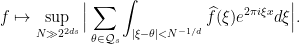
we notice that , with the Dirac delta supported in , and therefore this kernel has multiplier . This is a Weyl sum, a very well studied object for which we have plenty of results. The typical way to attack these sums is to use the Hardy-Littlewood circle method, which in this case allows us to replace the Weyl sum above by a more explicit one: in the case (for simplicity), we have that if is not “close” to a rational then the multiplier is extremely small, and viceversa if it is “close” to the rational then we can approximate the multiplier well by

The value of the latter expression is that the first factor does not depend on any longer, so that the dependence is isolated to the second factor; but this latter factor in turn has a nice expression as an oscillatory integral, which is much easier to treat than a Weyl sum. Indeed, it is so well behaved that we can essentially replace it by the characteristic function of the interval , for our purposes. Once we do this we can partition the rationals by dyadic size of their denominator, defining

and reduce to bound the maximal operators

(the factors 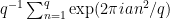can be absorbed into the function and efficiently estimated). We will have to sum in , but thanks to some decaying factors that I have conveniently left out it will suffice to prove that these operators are bounded with a norm that is at most (and notice , so that quantity is ). This is finally achieved through a very remarkable lemma, which is as follows:

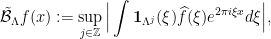
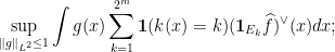
Lemma 1 [Bourgain]: Let be an integer and let a set of frequencies. Define the maximal frequency projections

where the supremum is restricted to those such that .
Then

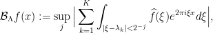
That the lemma allows one to conclude is evident. There are a few versions of this statement around, and I would like to clarify one thing: we can indeed remove the restriction on the supremum, if we reformulate the operator as follows. Given a finite set of frequencies, we let denote the -neighbourhood of the set , that is

Then if we redefine as

the conclusion of the lemma still holds, with the same constant.

I should remark here that actually this lemma is much more powerful than what one needs to run the above argument! Indeed, the rationals in lie on a regular lattice , where denotes the m.c.m. of all the integers between and ; moreover, replacing the oscillatory integral by a characteristic function was a bit rough, and one can more conveniently replace it by a smooth bump function instead. These two additional assumptions are enough to significantly simplify the proof of the lemma for the corresponding operator, as was noticed by Lacey some time later². This is another amazing thing that Bourgain typically did: he often proved stronger results than what he needed just because it didn’t occur to him that he could get away with less.

A final important remark about Bourgain’s lemma is that the logarithmic term in the constant is unavoidable. In particular, Bourgain, Kostyukovsky and Olevskiǐ proved that the constant must be at least using a beautiful construction based on the Kolmogorov rearrangement theorem. More on this in the future (but don’t hold your breath).

The trick this two-parts post is devoted to makes its appearance in the proof of the lemma above. In the next section we discuss a simpler but related result as a warmup.

2. Rademacher-Menshov theorem for frequency projections

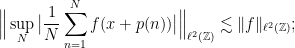
A standard result that might always come in handy when dealing with maximal frequency projections is a modern reformulation of a result by Rademacher and Menshov for orthonormal systems that goes by their names. The formulation we are interested in is the following:

Theorem 2 [Rademacher-Menshov à la Bourgain]: Let be a finite sequence of increasing measurable subsets of . The estimate

holds for any .

So, the maximal operator in the statement is a maximal frequency projection as well (notice the sets above are nested as well), but the constant this time depends on the range over which the supremum is taken and as such it cannot be applied to prove Bourgain’s lemma directly. However, the two results are quite related: indeed, let me remark that the Rademacher-Menshov theorem is actually used in the proof of the lemma for the operator , that is when the supremum is unrestricted; moreover, the proof of the boundedness of the simplified maximal operator of Lacey² rests heavily on the Rademacher-Menshov theorem as well.

There is also a slightly more general statement which is proven in a similar way and is useful in a variety of contexts:

Theorem 2′ [Rademacher-Menshov]: Let be a finite sequence of functions that satisfy

for any arbitrary choice of signs . Then for the maximal truncations of the estimate

holds.

It is almost immediate to verify that Theorem 2′ implies Theorem 2. We will illustrate both proofs, though they are really similar.

Let’s see how Bourgain proves Theorem 2. The overall strategy is to prove a bootstrap inequality, or self-improving inequality, for the optimal constant for which the inequality holds. This is overly fancy jargon to say a very simple (yet somewhat magical) thing: if you want to prove that , it is enough to prove for example that , or that , or anything of the form – this latter is perhaps most useful in conjunction with estimates and the use of Cauchy-Schwarz (it is for example how Bessel inequalities in time-frequency analysis are usually proved). Bear in mind that for these inequalities to make sense, you need to know somehow that the quantity is finite to begin with.

Proof of Theorem 2: We write as for shortness.
We can obviously assume that for convenience. We will prove the inequality dual to inequality (1), namely we will show that for all choices of

with ; this then implies (1). Indeed, observe that for any function there is a measurable function such that ; this is a trick known as the linearisation of the supremum (which I have already talked about in the past in the context of the Carleson operator). We can estimate the norm of this quantity by duality as

if we let then by Plancherel

The latter is bounded by (2) by , thus proving (1) conditional to (2).
Now we prove the dual inequality. Observe that a trivial use of the triangle inequality shows the constant is at most , so it is certainly finite and we want to obtain a good bound for it. For shortness, define and observe that if we have by Plancherel

With this information, we proceed to expand the square of the LHS of (2), obtaining

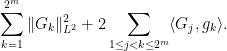
The first sum is bounded trivially by . For the second term, we bring the logarithm into the picture by expressing the indices in their binary form. Indeed, given two numbers written in their (binary) positional notation, how do you establish which one is larger? well, assuming that the strings you are given are of the same length, you start scanning from the leftmost digit to see whether they are the same, and as soon as you meet two distinct digits (a 1 and a 0), the string with digit 1 is the largest:

This suggests a way to reorganise the sum in such a way that the condition is automatically satisfied. We shift the indices back by 1 for convenience (that is they range over now). Any index corresponds uniquely to a string drawn from the alphabet through binary positional notation: precisely, corresponds to the string such that

We let be the set of all (finite) strings made of 0s and 1s and denote by the length of string . Given strings we can define the string to be the string obtained by appending to . Then we can define the set of strings of length with a given prefix: for such that , let

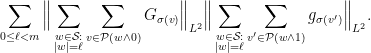
With this notation in place, we can rewrite the sum in terms of the length of the prefix and share when written in binary notation:

To be clear, and above have the same prefix but they differ in their -th digit from the left. In particular, has a 0 there whereas has a 1, and therefore automatically. Now we do Cauchy-Schwarz (twice) and bound the above by

The second factor is obviously bounded by ; for the first one, we apply the inequality (2) with the best constant for which it holds³, thus obtaining

Collecting everything together, if denotes the best constant for which (2) holds, the above has shown that

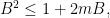
which, since is finite, shows that , as claimed.
[Observe that the gain came from the identity for , without which we would have had to bound both factors above by (2) thus gaining a factor of instead, which would have given us the useless inequality .]

Now, let’s see the proof of the more general Theorem 2′. At the heart of the proof there is the same idea of representing integers in their binary form; the proof however is now direct, so no dualisation and no bootstrap inequalities for the optimal constant.

Proof of theorem 2′:
Since we have the freedom of choosing the signs as we want, we have the ability to average over such choices. This is like a baby version of Khintchine’s inequality, except more trivial since we are in the case and we can just expand squares. We choose to average in dyadic blocks, that is in the following way. Assume of course that and for each define the partial sums

for . In other words, we are dividing up the range into consecutive blocks, each of length :

For each fixed we take the signs to be constant on each of these blocks – they can only differ if they belong to distinct blocks of length . Averaging over all these possible choices we get therefore that

Now we claim that we can bound the supremum pointwise by the sum of the square functions ; this will immediately conclude the proof by triangle inequality. The key to this last claim is again the fact that any integer can be written in binary form, that is as a sum of dyadic blocks. I will explain this formally, but the notation is a bit unwieldy: draw dyadic blocks on a line and the argument will be crystal clear. So, any 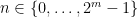can be written uniquely as

for a sequence of integers . Define the integer quantities as follows (we will need these to write the indices in correctly):

With this notation, you can verify easily that since

we have

By triangle inequality we have therefore

and since the RHS does not depend on we can take the supremum and conclude the claim.

This concludes part I of this two-part post. In the next part we will see how a similar (but crazier) idea to the one above – that of representing indices in positional notation – allows one to prove Lemma 1.

Appendix:
In this appendix we discuss how to obtain pointwise-a.e. convergence results in a dynamical system following Bourgain’s oscillation method. It is all nicely explained in Hands’ master thesis, and I am taking the presentation below from there (all eventual mistakes are mine though).
Suppose that the averages indeed do not converge everywhere. This means that the set

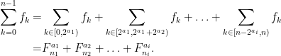
has positive -measure for any sufficiently small . In particular, by definition of , for any in this set there are increasing sequences such that for all we have 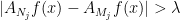– and in general these sequences depend on itself. We can make this a bit more explicit by saying that there are such that for the set

we have . It doesn’t matter what these numbers are, as long as they are positive. Notice that for any we can find an increasing sequence such that for any (and this is nothing but a reformulation of the condition above). However, this sequence again depends heavily on in general. We claim that, possibly losing a few points, we can choose a fixed sequence for which the above holds uniformly. We construct this sequence element by element as follows. Fix some value for and assume that we have chosen all elements up to included; we describe how to choose . Pick some and observe that by definition you can find such that ; we will impose that . Observe that for any we eventually pick subject to this constraint, there exists an index in such that (otherwise we would have by triangle inequality). Now we define the auxiliary sets

which are non-empty if by the previous discussion. We have that as , and therefore if we choose sufficiently large we will have . This is our choice of , and we pass to the construction of the next element in the sequence.
At the end of this procedure we have obtained an increasing sequence with the property that for every

An immediate consequence of this fact is that

which in turn shows that for any

as well. The precise lowerbound is irrelevant: what is important about this fact is that we have shown that there is an increasing sequence for which the latter quantity is bounded away from 0. So if we prove that for any increasing sequence the above must actually tend to 0, we will have reached a contradiction, showing that the sets have all zero measure and convergence happens a.e.. This is almost what Bourgain proves, but there is a further step (necessary or not, I don’t know, but I suspect it’s important): it suffices to treat the case where the suprema are restricted to a lacunary sequence with small lacunary constant. Precisely, for any (no relation to the previous one!), define the set

Bourgain shows that

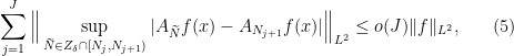
and this suffices to disprove (4) above. The reason is that we can always truncate our function and assume that ; and if we normalise we see that if is such that we have

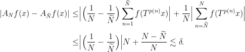
Thus we can replace any by a member of for an price. If the constants are chosen properly small, this is not an issue and one can indeed disprove (4) using (5) above.

Footnotes:
¹: The map is said to be weakly mixing if converges to in the Cesàro sense, that is .
²: Lacey’s maximal operator is as follows: let denote a function such that is a bump function with a minimum of regularity (more precisely, , , ). Let furthermore be fixed and let be a finite set of frequencies contained in the lattice . Lacey’s maximal operator is defined as

where the supremum is restricted to those such that . This operator actually satisfies an even better estimate, namely .
³: The first time you see this it looks like we are doing something illegal, using the very inequality we are trying to prove! However, as remarked at the beginning of the proof, the inequality is true with some large constant, and therefore there is an optimal constant for which it holds. We are allowed to use the inequality with the best constant even though we don’t yet know what that constant is!